{
"cells": [
{
"attachments": {},
"cell_type": "markdown",
"id": "5bd5782c",
"metadata": {},
"source": [
"# Method to help identify candidate features for RTS Consideration\n",
"\n",
"[Amazon Forecast](https://aws.amazon.com/forecast/) provides the ability to define and upload a special dataset type called [Related Time Series (RTS)](https://docs.aws.amazon.com/forecast/latest/dg/related-time-series-datasets.html) to help customers improve time-series model outcomes. RTS is a set of features that move in time, similar to the time movement of the Target Time Series (TTS) dataset. You may think of TTS as the dependent variable of the model and RTS as the independent variable(s). The goal of RTS is to help inform the model by explaining some of the variability in the dependent variable and produce a model with better accuracy.\n",
"\n",
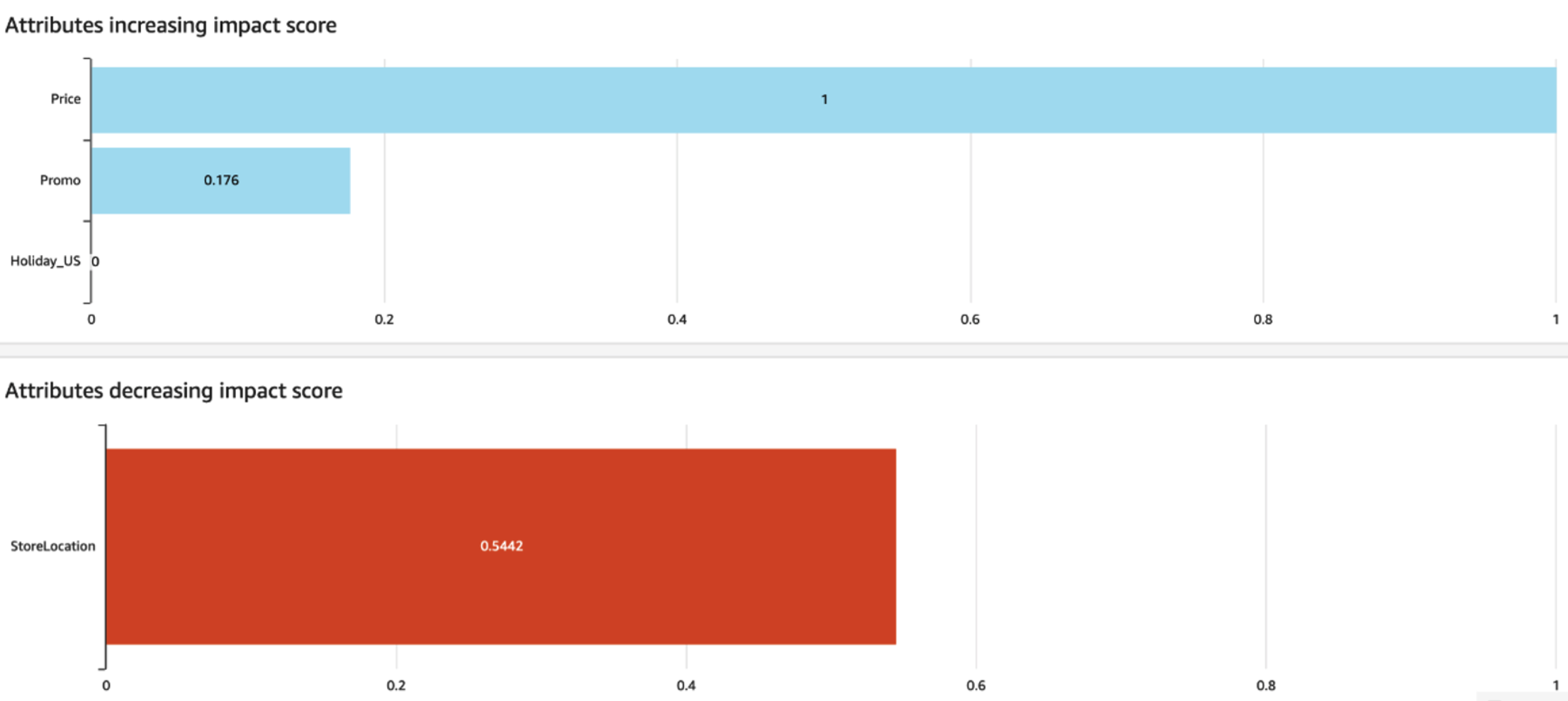
"When customers use RTS, Amazon Forecast has a feature called [Predictor Explainability](https://docs.aws.amazon.com/forecast/latest/dg/predictor-explainability.html) which provides both visual and tabular feedback on which data features in the RTS were helpful to inform the model as shown in Figure 1.
\n",
"\n",
"\n",
"**Figure 1 - Built-in Predictor Explainability in Amazon Forecast**\n",
"\n",
" \n",
"
\n",
"\n",
"## Motivation for an exploratory candidate feature selection method\n",
"\n",
"Sometimes customers have dozens or hundreds of candidate features of interest and ask for a quick way to help reduce the set by finding features that are not significant. At the same time, a mutually exclusive secondary ask exists. Customers want a method to identify independent RTS features that exhibit collinearity. When candidate features in the RTS have a strong relationship, it can put the overall model at risk of overfitting. The goal here is to remove all but one of the strongly correlated values.\n",
"\n",
"There are many ways to accomplish these tasks of candidate selection. The goal is to find features that help explain the TTS target value, but not explain other RTS variables. This notebook provides rule-of-thumb guidance to assist with candidate selection. You may choose to use other methods in addition to this method. After having pared down the candidate set, you can create a new RTS set and import it into Amazon Forecast, where the [AutoPredictor](https://aws.amazon.com/blogs/machine-learning/new-amazon-forecast-api-that-creates-up-to-40-more-accurate-forecasts-and-provides-explainability/) will give you more precise feedback. You can use the AutoPredictor metrics at the global or times-series level to understand if your proposed change was helpful and to what degree.\n",
"\n",
"Finally, to be explicit this notebook and candidate selection process has no temporal nature implied. This example simply compares the dependent and independent variables, **without time**, without sequence, and without any implied leads or lags."
]
},
{
"cell_type": "markdown",
"id": "16ad6356",
"metadata": {},
"source": [
"## Setup"
]
},
{
"cell_type": "code",
"execution_count": 1,
"id": "a7c9c8cb",
"metadata": {},
"outputs": [],
"source": [
"import pandas as pd\n",
"import numpy as np\n",
"import statsmodels.api as sm\n",
"pd.options.display.float_format = '{:.3f}'.format"
]
},
{
"cell_type": "markdown",
"id": "8265f656",
"metadata": {},
"source": [
"## Import RTS Data\n",
"\n",
"This section will load RTS data from an open-source data set and generate features that should be flagged by the candidate selection proposed."
]
},
{
"cell_type": "code",
"execution_count": 2,
"id": "e5663e5f",
"metadata": {},
"outputs": [
{
"name": "stdout",
"output_type": "stream",
"text": [
"(456547, 4)\n"
]
}
],
"source": [
"rts_column_list = [\"location_id\",\"item_id\",\"checkout_price\",\"base_price\",\n",
" \"emailer_for_promotion\",\"homepage_featured\",\"timestamp\"]\n",
"\n",
"rts_dtype_dic= { \"location_id\":str,\"item_id\":str,\"checkout_price\":float,\"base_price\":float,\n",
" \"emailer_for_promotion\":float,\"homepage_featured\":float,\"timestamp\":str}\n",
"\n",
"rts_index = ['timestamp','location_id','item_id']\n",
"\n",
"rts = pd.read_csv('./data/food-forecast-rts-uc1.csv',\n",
" index_col=rts_index,\n",
" skiprows=1,\n",
" names=rts_column_list,\n",
" dtype = rts_dtype_dic\n",
" )\n",
"print(rts.shape) "
]
},
{
"cell_type": "markdown",
"id": "831f37f9",
"metadata": {},
"source": [
"Next, features will be created to ensure they are flagged for low importance and collinearity:\n",
"- feature X1 is created to simulate noise, via a random function\n",
"- feature X2 is created to be highly correlated to base price\n",
"- feature X3 is an engineered feature to inform discounted sales price"
]
},
{
"cell_type": "code",
"execution_count": 3,
"id": "41806bd8",
"metadata": {},
"outputs": [],
"source": [
"# seed the pseudorandom number generator\n",
"from random import seed\n",
"from random import random\n",
"# seed random number generator\n",
"seed(42)\n",
"rts['x1'] = [np.random.normal() for k in rts.index]\n",
"rts['x2'] = rts['base_price']*0.9\n",
"rts['x3'] = rts['checkout_price']/rts['base_price']"
]
},
{
"cell_type": "markdown",
"id": "9d68e669",
"metadata": {},
"source": [
"Preview the RTS "
]
},
{
"cell_type": "code",
"execution_count": 4,
"id": "eaf2ac34",
"metadata": {},
"outputs": [
{
"data": {
"text/html": [
"
\n",
"\n",
"
\n",
" \n",
" \n",
" | \n",
" | \n",
" | \n",
" checkout_price | \n",
" base_price | \n",
" emailer_for_promotion | \n",
" homepage_featured | \n",
" x1 | \n",
" x2 | \n",
" x3 | \n",
"
\n",
" \n",
" timestamp | \n",
" location_id | \n",
" item_id | \n",
" | \n",
" | \n",
" | \n",
" | \n",
" | \n",
" | \n",
" | \n",
"
\n",
" \n",
" \n",
" \n",
" 2018-10-16 | \n",
" 10 | \n",
" 1062 | \n",
" 157.140 | \n",
" 157.140 | \n",
" 0.000 | \n",
" 0.000 | \n",
" 0.053 | \n",
" 141.426 | \n",
" 1.000 | \n",
"
\n",
" \n",
" 2018-10-30 | \n",
" 10 | \n",
" 1062 | \n",
" 158.170 | \n",
" 156.170 | \n",
" 0.000 | \n",
" 0.000 | \n",
" -1.791 | \n",
" 140.553 | \n",
" 1.013 | \n",
"
\n",
" \n",
" 2017-12-05 | \n",
" 10 | \n",
" 1062 | \n",
" 159.080 | \n",
" 182.390 | \n",
" 0.000 | \n",
" 0.000 | \n",
" 0.387 | \n",
" 164.151 | \n",
" 0.872 | \n",
"
\n",
" \n",
" 2017-03-21 | \n",
" 10 | \n",
" 1062 | \n",
" 159.080 | \n",
" 183.330 | \n",
" 0.000 | \n",
" 0.000 | \n",
" -0.658 | \n",
" 164.997 | \n",
" 0.868 | \n",
"
\n",
" \n",
" 2017-06-20 | \n",
" 10 | \n",
" 1062 | \n",
" 159.080 | \n",
" 183.360 | \n",
" 0.000 | \n",
" 0.000 | \n",
" -0.217 | \n",
" 165.024 | \n",
" 0.868 | \n",
"
\n",
" \n",
"
\n",
"
"
],
"text/plain": [
" checkout_price base_price \\\n",
"timestamp location_id item_id \n",
"2018-10-16 10 1062 157.140 157.140 \n",
"2018-10-30 10 1062 158.170 156.170 \n",
"2017-12-05 10 1062 159.080 182.390 \n",
"2017-03-21 10 1062 159.080 183.330 \n",
"2017-06-20 10 1062 159.080 183.360 \n",
"\n",
" emailer_for_promotion homepage_featured \\\n",
"timestamp location_id item_id \n",
"2018-10-16 10 1062 0.000 0.000 \n",
"2018-10-30 10 1062 0.000 0.000 \n",
"2017-12-05 10 1062 0.000 0.000 \n",
"2017-03-21 10 1062 0.000 0.000 \n",
"2017-06-20 10 1062 0.000 0.000 \n",
"\n",
" x1 x2 x3 \n",
"timestamp location_id item_id \n",
"2018-10-16 10 1062 0.053 141.426 1.000 \n",
"2018-10-30 10 1062 -1.791 140.553 1.013 \n",
"2017-12-05 10 1062 0.387 164.151 0.872 \n",
"2017-03-21 10 1062 -0.658 164.997 0.868 \n",
"2017-06-20 10 1062 -0.217 165.024 0.868 "
]
},
"execution_count": 4,
"metadata": {},
"output_type": "execute_result"
}
],
"source": [
"rts.head(5)"
]
},
{
"cell_type": "markdown",
"id": "dc2f23c4",
"metadata": {},
"source": [
"## Import TTS Data"
]
},
{
"cell_type": "code",
"execution_count": 5,
"id": "7701391a",
"metadata": {},
"outputs": [
{
"name": "stdout",
"output_type": "stream",
"text": [
"(456547, 1)\n"
]
}
],
"source": [
"tts_column_list = [\"location_id\",\"item_id\",\"target_value\",\"timestamp\"]\n",
"tts_dtype_dic= { \"location_id\":str,\"item_id\":str,\"target_value\":float,\"timestamp\":str}\n",
"tts_index = ['timestamp','location_id','item_id']\n",
"\n",
"tts = pd.read_csv('./data/food-forecast-tts-uc1.csv',\n",
" index_col=tts_index,\n",
" skiprows=1,\n",
" names=tts_column_list,\n",
" dtype = tts_dtype_dic\n",
" )\n",
"\n",
"print(tts.shape)"
]
},
{
"cell_type": "markdown",
"id": "12dac732",
"metadata": {},
"source": [
"Preview the TTS "
]
},
{
"cell_type": "code",
"execution_count": 6,
"id": "a827d339",
"metadata": {},
"outputs": [
{
"data": {
"text/html": [
"\n",
"\n",
"
\n",
" \n",
" \n",
" | \n",
" | \n",
" | \n",
" target_value | \n",
"
\n",
" \n",
" timestamp | \n",
" location_id | \n",
" item_id | \n",
" | \n",
"
\n",
" \n",
" \n",
" \n",
" 2016-11-08 | \n",
" 55 | \n",
" 1993 | \n",
" 270.000 | \n",
"
\n",
" \n",
" 2539 | \n",
" 189.000 | \n",
"
\n",
" \n",
" 2139 | \n",
" 54.000 | \n",
"
\n",
" \n",
" 2631 | \n",
" 40.000 | \n",
"
\n",
" \n",
" 1248 | \n",
" 28.000 | \n",
"
\n",
" \n",
"
\n",
"
"
],
"text/plain": [
" target_value\n",
"timestamp location_id item_id \n",
"2016-11-08 55 1993 270.000\n",
" 2539 189.000\n",
" 2139 54.000\n",
" 2631 40.000\n",
" 1248 28.000"
]
},
"execution_count": 6,
"metadata": {},
"output_type": "execute_result"
}
],
"source": [
"tts.head(5)"
]
},
{
"cell_type": "markdown",
"id": "b8ddc7bd",
"metadata": {},
"source": [
"## Merge the TTS and RTS\n",
"\n",
"Merge the two sets such that the Y and X values are in the same pandas row. To keep things simple, the composite key of item and location are blended into a single feature. You may choose to approach this in other ways."
]
},
{
"cell_type": "code",
"execution_count": 7,
"id": "37242eba",
"metadata": {},
"outputs": [],
"source": [
"merge_df = rts.join(tts)\n",
"merge_df = merge_df.reset_index()\n",
"\n",
"# create composite key for simplicity\n",
"merge_df['location_id']=merge_df['location_id'].astype(str)\n",
"merge_df['item_id']=merge_df['item_id'].astype(str)\n",
"merge_df[\"key\"] = merge_df[[\"location_id\", \"item_id\"]].apply(\"-\".join, axis=1)\n",
"\n",
"# delete original singleton columns, obsolete with composite\n",
"merge_df.drop(columns=['location_id','item_id'] , inplace=True)"
]
},
{
"cell_type": "code",
"execution_count": null,
"id": "a89d3d86",
"metadata": {},
"outputs": [],
"source": [
"# not needed, but if you want to ensure no time-series relatioships shuffle the data\n",
"#merge_df = merge_df.sample(frac=1, replace=True, random_state=1)"
]
},
{
"attachments": {},
"cell_type": "markdown",
"id": "e5b35839",
"metadata": {},
"source": [
"# Compute single regression per series\n",
"\n",
"This step computes a multivariate linear regression per each series. In this example, there are more than 3000 unique combinations of item and location originally. This step computes a regression for each. The time to complete will vary based on the size of your data, compute, and memory. As delivered, alpha 0.05 is used to test for significance."
]
},
{
"cell_type": "code",
"execution_count": 8,
"id": "8908c594",
"metadata": {},
"outputs": [],
"source": [
"setlist={}\n",
"i=0\n",
"\n",
"for ts in merge_df.key.unique():\n",
" \n",
" #create single ts dataframe\n",
" final_df = merge_df[merge_df['key']==ts]\n",
" \n",
" X=final_df\n",
" X=X.reset_index()\n",
" \n",
" y=X['target_value']\n",
" y=pd.DataFrame(y)\n",
" \n",
" X.drop(columns=['target_value','index','key','timestamp'], inplace=True)\n",
"\n",
" # produce regression for single time series in loop\n",
" model = sm.OLS(y,X)\n",
" results = model.fit()\n",
" results.params\n",
" \n",
" size=len(results.pvalues)\n",
"\n",
" # for each X variable in model, get statistics\n",
" for v in range(0,size):\n",
" \n",
" # tally for statistically signifiant using alpha 0.05\n",
" if results.pvalues[v]<=0.05:\n",
" s=1\n",
" else:\n",
" s=0\n",
" \n",
" list = {\n",
" 'key': ts,\n",
" 'variable': X.columns.values.tolist()[v],\n",
" 'coefficient': results.params[v],\n",
" 'p-value': results.pvalues[v],\n",
" 'significant': s,\n",
" 'count': 1\n",
" }\n",
" i=i+1\n",
" setlist[i] = list \n",
"\n",
"result = pd.DataFrame()\n",
"result = result.from_dict(setlist, \"index\")"
]
},
{
"attachments": {},
"cell_type": "markdown",
"id": "d97ea61b",
"metadata": {},
"source": [
"## How often do features significantly relate to the dependent variable?\n",
"\n",
"In the next cells, statistical significance by feature is computed by regression. The example highlights features that were significant in less than 20% of the time-series. You can change the over-under, but potentially these candidate RTS values can be eliminated as you propose the best set of values for RTS inclusion. Every use case is different; take care to change your over-under threshold."
]
},
{
"cell_type": "code",
"execution_count": 9,
"id": "4b76cba0",
"metadata": {},
"outputs": [
{
"name": "stdout",
"output_type": "stream",
"text": [
"Unique series in the dataset: 3597\n"
]
},
{
"data": {
"text/html": [
"\n",
"\n",
"
\n",
" \n",
" \n",
" | \n",
" significant | \n",
"
\n",
" \n",
" variable | \n",
" | \n",
"
\n",
" \n",
" \n",
" \n",
" x1 | \n",
" 181 | \n",
"
\n",
" \n",
"
\n",
"
"
],
"text/plain": [
" significant\n",
"variable \n",
"x1 181"
]
},
"execution_count": 9,
"metadata": {},
"output_type": "execute_result"
}
],
"source": [
"print('Unique series in the dataset:',result.key.nunique())\n",
"\n",
"regression_stats = pd.DataFrame(result.groupby('variable')['significant'].apply(lambda x : x.astype(int).sum()).sort_values())\n",
"regression_stats[regression_stats['significant']<=merge_df.key.nunique()*.2].sort_values(by=\"significant\")"
]
},
{
"attachments": {},
"cell_type": "markdown",
"id": "9b62c1b4",
"metadata": {},
"source": [
"In the above example, x1 was only significant in 192 of 3597 regressions. Remember, x1 was built from a random number, so it is expected for this feature to be called out here.
On the other hand; below, these fields appear significant in at least 20% or more series. Change the threshold as appropriate for your use case."
]
},
{
"cell_type": "code",
"execution_count": 10,
"id": "37dba986",
"metadata": {},
"outputs": [
{
"data": {
"text/html": [
"\n",
"\n",
"
\n",
" \n",
" \n",
" | \n",
" significant | \n",
"
\n",
" \n",
" variable | \n",
" | \n",
"
\n",
" \n",
" \n",
" \n",
" emailer_for_promotion | \n",
" 2052 | \n",
"
\n",
" \n",
" homepage_featured | \n",
" 2125 | \n",
"
\n",
" \n",
" x3 | \n",
" 2353 | \n",
"
\n",
" \n",
" checkout_price | \n",
" 2888 | \n",
"
\n",
" \n",
" base_price | \n",
" 3115 | \n",
"
\n",
" \n",
" x2 | \n",
" 3115 | \n",
"
\n",
" \n",
"
\n",
"
"
],
"text/plain": [
" significant\n",
"variable \n",
"emailer_for_promotion 2052\n",
"homepage_featured 2125\n",
"x3 2353\n",
"checkout_price 2888\n",
"base_price 3115\n",
"x2 3115"
]
},
"execution_count": 10,
"metadata": {},
"output_type": "execute_result"
}
],
"source": [
"regression_stats[regression_stats['significant']>merge_df.key.nunique()*.2].sort_values(by=\"significant\")"
]
},
{
"cell_type": "markdown",
"id": "b45d2708",
"metadata": {},
"source": [
"## Develop a Pearson correlation score for all bivariate pairs\n",
"The goal here is to identify high correlations between candidate X-values and remove them to prevent overfitting."
]
},
{
"cell_type": "code",
"execution_count": 11,
"id": "58c0adb0",
"metadata": {},
"outputs": [],
"source": [
"setlist={}\n",
"i=0\n",
"\n",
"for ts in merge_df.key.unique():\n",
" final_df = merge_df[merge_df['key']==ts]\n",
"\n",
" correlation_mat = final_df.corr()\n",
" strong_pairs = correlation_mat[(abs(correlation_mat) > 0.7) & (abs(correlation_mat)<1)]\n",
" strong_pairs = strong_pairs.reset_index().melt(id_vars='index')\n",
" strong_pairs = strong_pairs.dropna().reset_index()\n",
"\n",
" for v in range(1,strong_pairs.shape[0]):\n",
" \n",
" if not (strong_pairs['index'][v] !='target_value') or (strong_pairs['index'][v] != 'target_value'):\n",
" list = {\n",
" 'key': ts,\n",
" 'index': strong_pairs['index'][v],\n",
" 'variable': strong_pairs['variable'][v],\n",
" 'coefficient': strong_pairs['value'][v],\n",
" 'count': 1\n",
" }\n",
" i=i+1\n",
" setlist[i] = list \n",
" \n",
"result_corr = pd.DataFrame()\n",
"result_corr = result_corr.from_dict(setlist, \"index\")"
]
},
{
"cell_type": "markdown",
"id": "9f8f30c2",
"metadata": {},
"source": [
"## Inspect the Correlation Results\n",
"\n",
"As delivered, if more than 20% of the series are highly correlated, they are highlighted below. The idea is to apply business logic and domain knowledge to determine if one or more of these should be removed to prevent overfitting of the model.\n",
"\n",
"In this example, x2 was created as a function of price, which explains the high Pearson finding.\n",
"Variable x3 was created from other features too. Feature x3 represents a discounted price. It may be plausible to use this feature or the two features used to manufacture it -- but not both."
]
},
{
"cell_type": "code",
"execution_count": 12,
"id": "7bbaa15c",
"metadata": {},
"outputs": [
{
"data": {
"text/html": [
"\n",
"\n",
"
\n",
" \n",
" \n",
" | \n",
" index | \n",
" variable | \n",
" coefficient | \n",
"
\n",
" \n",
" \n",
" \n",
" 3 | \n",
" base_price | \n",
" x2 | \n",
" 1647 | \n",
"
\n",
" \n",
" 11 | \n",
" checkout_price | \n",
" x3 | \n",
" 2386 | \n",
"
\n",
" \n",
" 15 | \n",
" emailer_for_promotion | \n",
" x3 | \n",
" 811 | \n",
"
\n",
" \n",
" 34 | \n",
" x2 | \n",
" base_price | \n",
" 1321 | \n",
"
\n",
" \n",
" 42 | \n",
" x3 | \n",
" emailer_for_promotion | \n",
" 808 | \n",
"
\n",
" \n",
" 44 | \n",
" x3 | \n",
" target_value | \n",
" 720 | \n",
"
\n",
" \n",
"
\n",
"
"
],
"text/plain": [
" index variable coefficient\n",
"3 base_price x2 1647\n",
"11 checkout_price x3 2386\n",
"15 emailer_for_promotion x3 811\n",
"34 x2 base_price 1321\n",
"42 x3 emailer_for_promotion 808\n",
"44 x3 target_value 720"
]
},
"execution_count": 12,
"metadata": {},
"output_type": "execute_result"
}
],
"source": [
"stats = pd.DataFrame(result_corr.groupby(['index', 'variable'])[\"coefficient\"].apply(lambda x : x.astype(int).count())).reset_index()\n",
"stats[stats['coefficient']>=merge_df.key.nunique()*.2]"
]
}
],
"metadata": {
"kernelspec": {
"display_name": "conda_pytorch_p36",
"language": "python",
"name": "conda_pytorch_p36"
},
"language_info": {
"codemirror_mode": {
"name": "ipython",
"version": 3
},
"file_extension": ".py",
"mimetype": "text/x-python",
"name": "python",
"nbconvert_exporter": "python",
"pygments_lexer": "ipython3",
"version": "3.6.13"
}
},
"nbformat": 4,
"nbformat_minor": 5
}