Exoplanet Transit Method [via Chris Shallue]
" ] }, { "cell_type": "markdown", "metadata": {}, "source": [ "## Objective\n", "\n", "The Kepler spacecraft generated A LOT of data (over 650 GB of science data). Suppose we wanted to use a computer to find planet candidates from this data, but we don't have a labeled dataset. Perhaps we could pay graduate student to label 1000 time series sequences. Can we use this data of planet candidates to find other planet candidates and to distinguish planet candidates from other spurious signals collected by Kepler. This approach is similar to a traditional anomaly detection problem where we have example time series of normal machine operation. We can use the knowledge of normal behavior to identify abnormal behavior. Let's get started!" ] }, { "cell_type": "markdown", "metadata": {}, "source": [ "# Resources" ] }, { "cell_type": "markdown", "metadata": {}, "source": [ "* https://github.com/google-research/exoplanet-ml/tree/master/exoplanet-ml/astronet\n", "* Shallue, C. J., & Vanderburg, A. (2018). Identifying Exoplanets with Deep Learning: A Five-planet Resonant Chain around Kepler-80 and an Eighth Planet around Kepler-90. The Astronomical Journal, 155(2), 94.\n", "* https://exoplanets.nasa.gov/exoplanet-catalog/6128/kepler-90g/\n", "* https://exoplanets.nasa.gov/exoplanet-catalog/6129/kepler-90h/" ] }, { "cell_type": "markdown", "metadata": {}, "source": [ "Please use the tensorflow2.3 CPU / python 3.7 kernel with this notebook" ] }, { "cell_type": "code", "execution_count": null, "metadata": {}, "outputs": [], "source": [ "%pip install matplotlib seaborn" ] }, { "cell_type": "code", "execution_count": null, "metadata": {}, "outputs": [], "source": [ "# IMPORTS\n", "import tensorflow as tf\n", "import glob\n", "import numpy as np\n", "import pandas as pd\n", "import sagemaker\n", "from sagemaker.tensorflow import TensorFlow\n", "from sklearn.metrics import recall_score, classification_report, auc, roc_curve, precision_recall_curve, confusion_matrix\n", "from sklearn.model_selection import train_test_split\n", "from sklearn.metrics import f1_score\n", "import boto3\n", "import time \n", "import matplotlib.pyplot as plt\n", "import seaborn as sns\n", "from IPython.display import display, clear_output" ] }, { "cell_type": "markdown", "metadata": {}, "source": [ "# Data\n", "\n", "For this workshop we will use data that has been prepared, transformed, and cleaned. We will use a 1000 time series signals of planet cadidates. This could have been labeled using graduate students using our hypothetical example. Each time series has been scaled and centered, and includes a 'global' 2001 timestamp series and a 'local' 201 timestamp series. " ] }, { "cell_type": "markdown", "metadata": {}, "source": [ "## Download Dataset" ] }, { "cell_type": "code", "execution_count": null, "metadata": {}, "outputs": [], "source": [ "# Download compressed archive (~138MB).\n", "!mkdir data \n", "!aws s3 cp s3://aws-machine-learning-immersion-day/kepler-tce-tfrecords-20180220.tar ./data/" ] }, { "cell_type": "code", "execution_count": null, "metadata": {}, "outputs": [], "source": [ "!mkdir data/processed\n", "!tar -xvf ./data/kepler-tce-tfrecords-20180220.tar -C ./data/processed/ --no-same-owner" ] }, { "cell_type": "code", "execution_count": null, "metadata": {}, "outputs": [], "source": [ "files = glob.glob('./data/processed/tfrecord/train*')\n", "files" ] }, { "cell_type": "markdown", "metadata": {}, "source": [ "## Configure SageMaker" ] }, { "cell_type": "code", "execution_count": null, "metadata": {}, "outputs": [], "source": [ "sess = sagemaker.Session()\n", "role = sagemaker.get_execution_role()\n", "bucket_name = sagemaker.Session().default_bucket()\n", "\n", "prefix = 'remars.exoplanet'" ] }, { "cell_type": "markdown", "metadata": {}, "source": [ "Terminology:\n", "\n", "* TCE = Threshold Crossing Events\n", "* PC = Planet Candidate\n", "* NTP = Astrophysical False Positive - not planet\n", "* AFP = Nontransiting Phenomenon - not planet\n", "\n", "The predictions can be PC, NTP, or AFP\n" ] }, { "cell_type": "code", "execution_count": null, "metadata": {}, "outputs": [], "source": [ "tfrecord_format = {\n", " \"av_pred_class\": tf.io.FixedLenFeature([], tf.string),\n", " \"av_training_set\": tf.io.FixedLenFeature([], tf.string),\n", " \"global_view\": tf.io.FixedLenFeature([2001], tf.float32),\n", " \"local_view\": tf.io.FixedLenFeature([201],tf.float32),\n", " \"kepid\": tf.io.FixedLenFeature([],tf.int64),\n", " \"spline_bkspace\": tf.io.FixedLenFeature([],tf.float32),\n", " \"tce_depth\": tf.io.FixedLenFeature([],tf.float32),\n", " \"tce_duration\": tf.io.FixedLenFeature([],tf.float32),\n", " \"tce_impact\": tf.io.FixedLenFeature([],tf.float32),\n", " \"tce_max_mult_ev\": tf.io.FixedLenFeature([],tf.float32),\n", " \"tce_model_snr\": tf.io.FixedLenFeature([],tf.float32),\n", " \"tce_period\": tf.io.FixedLenFeature([],tf.float32),\n", " \"tce_plnt_num\": tf.io.FixedLenFeature([],tf.int64),\n", " \"tce_prad\": tf.io.FixedLenFeature([],tf.float32),\n", " \"tce_time0bk\": tf.io.FixedLenFeature([],tf.float32)\n", " }" ] }, { "cell_type": "code", "execution_count": null, "metadata": {}, "outputs": [], "source": [ "# Read the data back out.\n", "def decode_fn(record_bytes):\n", " return tf.io.parse_single_example(\n", " # Data\n", " record_bytes,\n", " # Schema\n", " tfrecord_format\n", " )" ] }, { "cell_type": "code", "execution_count": null, "metadata": {}, "outputs": [], "source": [ "%%time\n", "c = []\n", "pc_global = []\n", "pc_local = []\n", "non_pc_global = []\n", "non_pc_local = []\n", "for rec in tf.data.TFRecordDataset(files).map(decode_fn):\n", " c.append(rec['av_pred_class'].numpy().decode('utf-8'))\n", " if 'PC' in rec['av_pred_class'].numpy().decode('utf-8'):\n", " pc_global.append(rec[\"global_view\"].numpy())\n", " pc_local.append(rec[\"local_view\"].numpy())\n", " else:\n", " non_pc_global.append(rec[\"global_view\"].numpy())\n", " non_pc_local.append(rec[\"local_view\"].numpy())\n", " \n", " if (rec[\"kepid\"].numpy() == 11442793 and\n", " rec[\"tce_plnt_num\"].numpy() == 1):\n", " kepler = rec\n", " if 'NTP' in rec['av_pred_class'].numpy().decode('utf-8'):\n", " ntp = rec\n", " if 'AFP' in rec['av_pred_class'].numpy().decode('utf-8'): \n", " afp = rec" ] }, { "cell_type": "code", "execution_count": null, "metadata": {}, "outputs": [], "source": [ "print(f\"Total number of planet candidates {c.count('PC')}\") \n", "print(f\"Total number of non planet candidates {len(c) - c.count('PC')}\")" ] }, { "cell_type": "markdown", "metadata": {}, "source": [ "## Visualization\n", "\n", "Let's take a look at a single planet candidate. Here is an example of [Kepler-90](https://exoplanets.nasa.gov/exoplanet-catalog/6128/kepler-90g/) This is a G-type star in the Constellation Draco and is 2840 light years from Earth. " ] }, { "cell_type": "code", "execution_count": null, "metadata": {}, "outputs": [], "source": [ "# Plot the global and local views.\n", "global_view = np.array(kepler[\"global_view\"].numpy())\n", "local_view = np.array(kepler[\"local_view\"].numpy())\n", "fig, axes = plt.subplots(1, 2, figsize=(20, 6))\n", "axes[0].plot(global_view, \".\")\n", "axes[1].plot(local_view, \".\")\n", "axes[0].title.set_text('planet candidate - global view')\n", "axes[1].title.set_text('planet candidate - local view')\n", "plt.show()" ] }, { "cell_type": "code", "execution_count": null, "metadata": {}, "outputs": [], "source": [ "# Plot the global and local views.\n", "global_view = np.array(ntp[\"global_view\"].numpy())\n", "local_view = np.array(ntp[\"local_view\"].numpy())\n", "fig, axes = plt.subplots(1, 2, figsize=(20, 6))\n", "axes[0].plot(global_view, \".\")\n", "axes[1].plot(local_view, \".\")\n", "axes[0].title.set_text('non transiting phenomenon - global view')\n", "axes[1].title.set_text('non transiting phenomenon - local view')\n", "plt.show()" ] }, { "cell_type": "code", "execution_count": null, "metadata": {}, "outputs": [], "source": [ "# Plot the global and local views.\n", "global_view = np.array(afp[\"global_view\"].numpy())\n", "local_view = np.array(afp[\"local_view\"].numpy())\n", "fig, axes = plt.subplots(1, 2, figsize=(20, 6))\n", "axes[0].plot(global_view, \".\")\n", "axes[1].plot(local_view, \".\")\n", "axes[0].title.set_text('astrophysical false positive - global view')\n", "axes[1].title.set_text('astrophysical false positive - local view')\n", "plt.show()" ] }, { "cell_type": "markdown", "metadata": {}, "source": [ "## Train | Validation Split" ] }, { "cell_type": "markdown", "metadata": {}, "source": [ "In this example, let's assume that we have 12000 example time series and we want to find the planet candidates. Let's also assume that we don't have labeled data. How do we approach a problem like this? Our grad students identified 1000 planet candidates. We'll use this data to label the remaining dataset. Or said, differently, we'll use this data to determine other planet candidates and non planet candidates. We will concatenate the local and global views together into a single 2202 timestamp time series." ] }, { "cell_type": "code", "execution_count": null, "metadata": {}, "outputs": [], "source": [ "pc_local_numpy = np.array(pc_local)\n", "pc_global_numpy = np.array(pc_global)\n", "temp = np.concatenate((pc_global_numpy,pc_local_numpy),axis=1)" ] }, { "cell_type": "code", "execution_count": null, "metadata": {}, "outputs": [], "source": [ "# get 1000 samples of planet candidates\n", "temp, temp_ = train_test_split(\n", " temp, \n", " train_size=1000, \n", " random_state=4321, \n", " shuffle=True)" ] }, { "cell_type": "code", "execution_count": null, "metadata": {}, "outputs": [], "source": [ "non_pc_local_numpy = np.array(non_pc_local)\n", "non_pc_global_numpy = np.array(non_pc_global)\n", "temp_non = np.concatenate((non_pc_global_numpy,non_pc_local_numpy),axis=1)" ] }, { "cell_type": "code", "execution_count": null, "metadata": {}, "outputs": [], "source": [ "labels = [1]*len(temp_)+[0]*len(temp_non)" ] }, { "cell_type": "code", "execution_count": null, "metadata": {}, "outputs": [], "source": [ "temp_ = np.concatenate((temp_,temp_non),axis=0)" ] }, { "cell_type": "code", "execution_count": null, "metadata": {}, "outputs": [], "source": [ "# split data into 80% training, 20% validation\n", "train, validation = train_test_split(\n", " temp, \n", " test_size=.2, \n", " random_state=4321, \n", " shuffle=True)" ] }, { "cell_type": "code", "execution_count": null, "metadata": {}, "outputs": [], "source": [ "print(f'Training dataset shape: {train.shape}')\n", "print(f'Validation dataset shape: {validation.shape}')" ] }, { "cell_type": "code", "execution_count": null, "metadata": {}, "outputs": [], "source": [ "np.savez('./data/training', train=train)\n", "np.savez('./data/validation', validation=validation)" ] }, { "cell_type": "markdown", "metadata": {}, "source": [ "Upload datasets to S3" ] }, { "cell_type": "code", "execution_count": null, "metadata": {}, "outputs": [], "source": [ "training_input_path = sess.upload_data('data/training.npz', bucket=bucket_name, key_prefix=prefix+'/training')\n", "validation_input_path = sess.upload_data('data/validation.npz', bucket=bucket_name, key_prefix=prefix+'/validation')\n", "print('Uploaded training data location: {}'.format(training_input_path))\n", "print('Uploaded validation data location: {}'.format(validation_input_path))" ] }, { "cell_type": "markdown", "metadata": {}, "source": [ "# Model Training\n", "\n", "## Autoencoder\n", "\n", "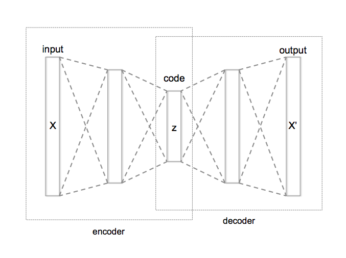\n", "\n", "AutoEncoders are a special kind of neural network, where your input is 'x' and your output is 'x' as well. What this really means is that we are trying to learn a function, where the input and output are the same. In a linear system an autoencoder would be the identity matrix, however, we are going to use a non-linear neural network to construct our autoencoder. \n", "\n", "The function f(x), that we are going to learn is approximately equal to x\n", "\n", "Few things to note.\n", "\n", "* We are reducing the number of nodes in the hidden layers, which will force the network to learn the features from the dataset. Intuition being that this \"code\" is a set of abstracted features which represents or creates a fingerprint for the training dataset.\n", "* Since we are starting with the input 'x', reducing into a abstracted features and then reconstructing back the 'x' means we don't need a labeled dataset. We are converting the problem from an usupervised problem to a supervised problem. \n", "* The \"code\" is intutively a representation of abstracted features.\n", "\n", "For our explanet dataset, we are going a dataset of 1000 time series that have been identified as 'planet cadidates'. We will train the autoencoder on this data. Next, we'll used the trained network to analyze a larger dataset. We will use the reconstruction error (Mean Squared Error - MSE) to find other planet crossing data. During this process the network should try to learn a unique representation of what a planet candidate time series looks like. " ] }, { "cell_type": "code", "execution_count": null, "metadata": {}, "outputs": [], "source": [ "output_location = f's3://{bucket_name}/{prefix}/output'\n", "\n", "print('Training artifacts will be uploaded to: {}'.format(output_location))" ] }, { "cell_type": "code", "execution_count": null, "metadata": {}, "outputs": [], "source": [ "!pygmentize ./code/autoencoder.fc.py" ] }, { "cell_type": "code", "execution_count": null, "metadata": {}, "outputs": [], "source": [ "tf_estimator = TensorFlow(entry_point='./code/autoencoder.fc.py', \n", " role=role,\n", " instance_count=1, \n", " instance_type='ml.m5.xlarge',\n", " framework_version='2.2', \n", " py_version='py37',\n", " script_mode=True,\n", "# use_spot_instances=True,\n", "# max_run=3600,\n", "# max_wait=3600,\n", " hyperparameters={\n", " 'epochs': 30,\n", " 'batch-size': 64}\n", " )" ] }, { "cell_type": "code", "execution_count": null, "metadata": {}, "outputs": [], "source": [ "tf_estimator.fit({'training': training_input_path, 'validation': validation_input_path})" ] }, { "cell_type": "code", "execution_count": null, "metadata": {}, "outputs": [], "source": [ "# plot validation and training progress\n", "client = boto3.client('logs')\n", "BASE_LOG_NAME = '/aws/sagemaker/TrainingJobs'\n", "\n", "def plot_log(model):\n", " logs = client.describe_log_streams(logGroupName=BASE_LOG_NAME, logStreamNamePrefix=model._current_job_name)\n", " cw_log = client.get_log_events(logGroupName=BASE_LOG_NAME, logStreamName=logs['logStreams'][0]['logStreamName'])\n", "\n", " val = []\n", " train = []\n", " iteration = []\n", " count = 0\n", " for e in cw_log['events']:\n", " msg = e['message']\n", " if 's - loss:' in msg:\n", " msg = msg.split(' ')\n", " #print(msg)\n", " train.append(float(msg[5]))\n", " val.append(float(msg[8]))\n", " iteration.append(count)\n", " count+=1\n", "\n", " fig, ax = plt.subplots(figsize=(15,5))\n", " plt.xlabel('Epoch')\n", " plt.ylabel('Error')\n", " train_plot, = ax.plot(iteration, train, label='train')\n", " val_plot, = ax.plot(iteration, val, label='validation')\n", " plt.legend(handles=[train_plot,val_plot])\n", " plt.grid()\n", " plt.show()\n", "\n" ] }, { "cell_type": "code", "execution_count": null, "metadata": {}, "outputs": [], "source": [ "plot_log(tf_estimator)" ] }, { "cell_type": "markdown", "metadata": {}, "source": [ "# Deploy" ] }, { "cell_type": "code", "execution_count": null, "metadata": {}, "outputs": [], "source": [ "%%time\n", "\n", "tf_endpoint_name = 'remars-autoencoder-'+time.strftime(\"%Y-%m-%d-%H-%M-%S\", time.gmtime())\n", "\n", "tf_predictor = tf_estimator.deploy(initial_instance_count=1,\n", " instance_type='ml.m5.xlarge', \n", " endpoint_name=tf_endpoint_name) " ] }, { "cell_type": "code", "execution_count": null, "metadata": {}, "outputs": [], "source": [ "## How do you connect to an already deployed endpoint\n", "# end_point_name = 'ENDPOINT_NAME'\n", "# tf_predictor = sagemaker.tensorflow.model.TensorFlowPredictor(end_point_name,sagemaker_session=sess)" ] }, { "cell_type": "markdown", "metadata": {}, "source": [ "# Evaluate" ] }, { "cell_type": "markdown", "metadata": {}, "source": [ "## single prediction" ] }, { "cell_type": "code", "execution_count": null, "metadata": {}, "outputs": [], "source": [ "validation[1,:]" ] }, { "cell_type": "code", "execution_count": null, "metadata": {}, "outputs": [], "source": [ "a = tf_predictor.predict(validation[1,:]);" ] }, { "cell_type": "code", "execution_count": null, "metadata": {}, "outputs": [], "source": [ "plt.plot(validation[1,:],'b*',a['predictions'][0],'r*')\n", "plt.legend(('actual','prediction'))" ] }, { "cell_type": "markdown", "metadata": {}, "source": [ "## hold out dataset prediction" ] }, { "cell_type": "code", "execution_count": null, "metadata": {}, "outputs": [], "source": [ "def predict(data, rows=500):\n", " split_array = np.array_split(data, int(data.shape[0] / float(rows) + 1))\n", " predictions = []\n", " for array in split_array:\n", " predictions.extend(tf_predictor.predict(array)['predictions'])\n", "\n", " return predictions" ] }, { "cell_type": "code", "execution_count": null, "metadata": {}, "outputs": [], "source": [ "%%time\n", "train_pred = predict(train)\n", "val_pred = predict(validation)\n", "pred_ = predict(temp_)" ] }, { "cell_type": "code", "execution_count": null, "metadata": {}, "outputs": [], "source": [ "train_mse = np.mean(np.power(train - train_pred, 2), axis=1)\n", "val_mse = np.mean(np.power(validation - val_pred, 2), axis=1)\n", "mse_ = np.mean(np.power(temp_ - pred_, 2), axis=1)" ] }, { "cell_type": "code", "execution_count": null, "metadata": {}, "outputs": [], "source": [ "error_df_val = pd.DataFrame({'reconstruction_error': val_mse})\n", "error_df_val.describe(percentiles=[.50,.90,.95,.99,.999,.9999])" ] }, { "cell_type": "code", "execution_count": null, "metadata": {}, "outputs": [], "source": [ "fig = plt.figure(figsize=(15,10))\n", "ax = fig.add_subplot(111)\n", "_ = ax.hist(val_mse, bins=100, range=(0,1),density=True,color='blue',edgecolor='black',alpha=0.6,label='validation')\n", "_ = ax.hist(mse_, bins=100, range=(0,1),density=True,color='red',edgecolor='black',alpha=0.4,label='hold_out')\n", "plt.legend()\n", "plt.xlabel('reconstruction error, MSE')\n", "plt.ylabel('normalized count')\n" ] }, { "cell_type": "markdown", "metadata": {}, "source": [ "We can see from the reconstruction mean squared error above the validation data and the hold out data are different. While there are some examples in the hold out dataset that have a near zero mean squared error, there are also some that have much higher reconstruction error. The hold out dataset with MSE near zero is likely planet candidates and the time series with MSE greater than 0.1 are likely the non planet candidates. " ] }, { "cell_type": "code", "execution_count": null, "metadata": {}, "outputs": [], "source": [ "# apply threshold \n", "def to_labels(pos_probs, threshold):\n", " return (pos_probs <= threshold).astype('int')" ] }, { "cell_type": "code", "execution_count": null, "metadata": {}, "outputs": [], "source": [ "fpr, tpr, thresholds = roc_curve(labels,mse_,pos_label=0)\n", "roc_auc = auc(fpr, tpr)\n", "\n", "plt.title('Receiver Operating Characteristic')\n", "plt.plot(fpr, tpr, label='AUC = %0.4f'% roc_auc)\n", "plt.legend(loc='lower right')\n", "plt.plot([0,1],[0,1],'r--')\n", "plt.xlim([-0.001, 1])\n", "plt.ylim([0, 1.001])\n", "plt.ylabel('True Positive Rate')\n", "plt.xlabel('False Positive Rate')\n", "plt.show();\n" ] }, { "cell_type": "code", "execution_count": null, "metadata": {}, "outputs": [], "source": [ "precision, recall, th = precision_recall_curve(labels, mse_, pos_label=0)\n", "plt.plot(recall, precision, 'b', label='Precision-Recall curve')\n", "plt.title('Recall vs Precision')\n", "plt.xlabel('Recall')\n", "plt.ylabel('Precision')\n", "plt.show()" ] }, { "cell_type": "code", "execution_count": null, "metadata": {}, "outputs": [], "source": [ "plt.plot(th, precision[1:], 'b', label='Threshold-Precision curve')\n", "plt.title('Precision for different threshold values')\n", "plt.xlabel('Threshold')\n", "plt.ylabel('Precision')\n", "plt.xlim((0,.2))\n", "plt.show()" ] }, { "cell_type": "code", "execution_count": null, "metadata": {}, "outputs": [], "source": [ "plt.plot(th, recall[1:], 'b', label='Threshold-Recall curve')\n", "plt.title('Recall for different threshold values')\n", "plt.xlabel('Threshold')\n", "plt.ylabel('Recall')\n", "plt.xlim((0,.2))\n", "plt.show()" ] }, { "cell_type": "code", "execution_count": null, "metadata": {}, "outputs": [], "source": [ "# define thresholds\n", "thresholds = np.arange(0, 0.2, 0.001)\n", "# evaluate each threshold\n", "scores = [f1_score(labels, to_labels(mse_, t)) for t in thresholds]\n", "# get best threshold\n", "ix = np.argmax(scores)\n", "print('Threshold=%.3f, F-Score=%.5f' % (thresholds[ix], scores[ix]))" ] }, { "cell_type": "code", "execution_count": null, "metadata": {}, "outputs": [], "source": [ "plt.plot(thresholds, scores, 'b', label='F1 curve')\n", "plt.title('F1 for different threshold values')\n", "plt.xlabel('Threshold')\n", "plt.ylabel('F1')\n", "#plt.xlim((0,.2))\n", "plt.show()" ] }, { "cell_type": "code", "execution_count": null, "metadata": {}, "outputs": [], "source": [ "thresh = 0.1" ] }, { "cell_type": "code", "execution_count": null, "metadata": {}, "outputs": [], "source": [ "class_list = ['NOT PC', 'PC']\n", "fig, ax = plt.subplots(figsize=(15,10))\n", "cm = confusion_matrix(labels,to_labels(mse_,thresh))\n", "normalized_cm = cm.astype('float') / cm.sum(axis=1)[:, np.newaxis]\n", "sns.heatmap(normalized_cm, ax=ax, annot=cm, fmt='',xticklabels=class_list,yticklabels=class_list)\n", "plt.xlabel('Predicted')\n", "plt.ylabel('Actual')\n", "plt.title('Confusion Matrix')\n", "plt.show()" ] }, { "cell_type": "markdown", "metadata": {}, "source": [ "If we use a threshold of 0.1 we can try to seperate out additional timeseries that are not planet crosssing. Again, recall that we trained the network on planet candidates and timeseries that have high reconstruction error exhibit different behavior than the planet candidates. When we use a threshold of 0.1 we identify ~3000 timeseries that are NOT planet candidates. Similarly we could look for timeseries that have near zero reconstruction error to identify series of additional planet candidates. " ] }, { "cell_type": "code", "execution_count": null, "metadata": {}, "outputs": [], "source": [ "print(\"Classification Report: \")\n", "print(classification_report(y_true=labels, y_pred=to_labels(mse_,thresh)))" ] }, { "cell_type": "markdown", "metadata": {}, "source": [ "# Conclusion and Call to Action" ] }, { "cell_type": "markdown", "metadata": {}, "source": [ "We've shown above how to train a fully connected feed forward autoencoder. In this approach we concatenated the two time series. We used the reconstruction error to seperate the planet candidates from non planet cadidates. However, we can also use an autoencoder architecture with a convolution or recurrent approach. Using this notebook as a starting point, compare and contrast the performance of the fully connected autoencoder with a convolution or recurrent approach. " ] }, { "cell_type": "markdown", "metadata": {}, "source": [ "## Clean up" ] }, { "cell_type": "code", "execution_count": null, "metadata": {}, "outputs": [], "source": [ "tf_predictor.delete.endpoint()" ] } ], "metadata": { "instance_type": "ml.t3.medium", "kernelspec": { "display_name": "Python 3 (TensorFlow 2.3 Python 3.7 CPU Optimized)", "language": "python", "name": "python3__SAGEMAKER_INTERNAL__arn:aws:sagemaker:us-east-1:081325390199:image/tensorflow-2.3-cpu-py37-ubuntu18.04-v1" }, "language_info": { "codemirror_mode": { "name": "ipython", "version": 3 }, "file_extension": ".py", "mimetype": "text/x-python", "name": "python", "nbconvert_exporter": "python", "pygments_lexer": "ipython3", "version": "3.7.10" } }, "nbformat": 4, "nbformat_minor": 5 }