00\_SageMakerAlgo
================

Clear the workspace

``` r
rm(list = ls())
```

Installing and loading the packages needed for this notebook

``` r
if (!'Metrics' %in% installed.packages()) {install.packages("Metrics")}
if (!'tidyverse' %in% installed.packages()) {install.packages("tidyverse")}
if (!'caret' %in% installed.packages()) {install.packages("caret")}

suppressWarnings(library(reticulate))
suppressWarnings(library(readr))
suppressWarnings(library(ggplot2))
suppressWarnings(library(dplyr))
suppressWarnings(library(stringr))
suppressWarnings(library(Metrics))
suppressWarnings(library(tidyverse))
suppressWarnings(library(caret))
suppressWarnings(library(pROC))
```

Next, loading the Reticulate library and import the SageMaker Python
module. Reticulate provides interface to ‘Python’ modules, classes, and
functions.

Amazon SageMaker Python SDK is an open source library for training and
deploying machine-learned models on Amazon SageMaker. With the SDK, you
can train and deploy models using popular deep learning frameworks,
algorithms provided by Amazon, or your own algorithms built into
SageMaker-compatible Docker images.
<https://sagemaker.readthedocs.io/en/stable/>

``` r
library(reticulate)
sagemaker <- import('sagemaker')
session <- sagemaker$Session()
bucket <- session$default_bucket()
role_arn <- sagemaker$get_execution_role()
print(role_arn)
```

Reading the data file churn.txt. The data is for customer churn in a
telecommunication organization (synthetic data). The goal is to predict
whether a customer is going to churn or not.

``` r
sagemaker$s3$S3Downloader$download("s3://sagemaker-sample-files/datasets/tabular/synthetic/churn.txt", "dataset")
churn <- read_csv(file = "dataset/churn.txt", col_names = TRUE, show_col_types = FALSE)
head(churn)
```

    ## # A tibble: 6 × 21
    ##   State `Account Length` `Area Code` Phone    `Int'l Plan` `VMail Plan`
    ##   <chr>            <dbl>       <dbl> <chr>    <chr>        <chr>       
    ## 1 PA                 163         806 403-2562 no           yes         
    ## 2 SC                  15         836 158-8416 yes          no          
    ## 3 MO                 131         777 896-6253 no           yes         
    ## 4 WY                  75         878 817-5729 yes          yes         
    ## 5 WY                 146         878 450-4942 yes          no          
    ## 6 VA                  83         866 454-9110 no           no          
    ## # … with 15 more variables: VMail Message <dbl>, Day Mins <dbl>,
    ## #   Day Calls <dbl>, Day Charge <dbl>, Eve Mins <dbl>, Eve Calls <dbl>,
    ## #   Eve Charge <dbl>, Night Mins <dbl>, Night Calls <dbl>, Night Charge <dbl>,
    ## #   Intl Mins <dbl>, Intl Calls <dbl>, Intl Charge <dbl>, CustServ Calls <dbl>,
    ## #   Churn? <chr>

Carrying out various data preprocessing steps

``` r
#Transforming the categorical variables to dummy variables since Xgboost only takes numerical inputs for features
#Now dropping certain columns that are redundant using dplyr's select method
churn = select(churn, -c("Phone", "Day Charge", "Eve Charge", "Night Charge", "Intl Charge"))

churn <- rename(churn, "intlplan" = "Int'l Plan")
churn <- rename(churn, "churn" = "Churn?")
```

Plotting international plan histogram as a function of target variable
“churn” using ggplot2

``` r
ggplot(churn, aes(x = churn, fill = intlplan)) +  geom_bar() + theme_classic()
```

![](00_SageMakerAlgo_files/figure-gfm/unnamed-chunk-6-1.png)<!-- -->

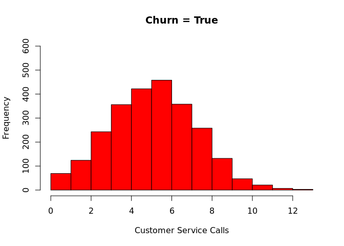
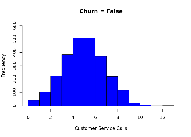
Plotting histograms for customer service calls as a function of target
variable (churn), using R’s hist function

``` r
hist(churn$"CustServ Calls"[which(churn$churn == "True.")], col = 'red', breaks = 15, ylim = c(0,600), main = "Churn = True", xlab = "Customer Service Calls")
```

![](00_SageMakerAlgo_files/figure-gfm/unnamed-chunk-7-1.png)<!-- -->

``` r
hist(churn$"CustServ Calls"[which(churn$churn == "False.")], col = 'blue', breaks = 15, ylim = c(0,600),main = "Churn = False", xlab = "Customer Service Calls")
```

![](00_SageMakerAlgo_files/figure-gfm/unnamed-chunk-7-2.png)<!-- -->

Additional pre-processing steps

``` r
#Changing target variable churn into dummy variable and keeping just True column while dropping False
churn <- churn %>% mutate(dummy=1) %>% spread(key="churn",value=dummy, fill=0)
churn <- subset(churn, select = -c(False.))
churn <- rename(churn, "churn" = True.)

#Making the target variable "churn" as the first column as XGBoost expects the data to be in this format
churn <- churn %>% select("churn", everything())

#Transforming intlplan (international plan) to dummy, dropping resulting "no" variable and renaming "yes" using dplyr's rename method
churn <- churn %>% mutate(dummy=1) %>% spread(key="intlplan",value=dummy, fill=0)
churn <- subset(churn, select = -c(no))
churn <- rename(churn, "intlplan" = yes)

#Transforming VMaill plan to dummy, dropping resulting "no" variable and renaming "yes" using dplyr's rename method
churn <- churn %>% mutate(dummy=1) %>% spread(key="VMail Plan",value=dummy, fill=0)
churn <- subset(churn, select = -c(no))
churn <- rename(churn, "VMail plan" = yes)

#Transforming variable "State" into dummy variables
churn <- churn %>% mutate(dummy=1) %>% spread(key="State",value=dummy, fill=0)
head(churn)
```

    ## # A tibble: 6 × 66
    ##   churn `Account Length` `Area Code` `VMail Message` `Day Mins` `Day Calls`
    ##   <dbl>            <dbl>       <dbl>           <dbl>      <dbl>       <dbl>
    ## 1     1              163         806             300       8.16           3
    ## 2     0               15         836               0      10.0            4
    ## 3     0              131         777             300       4.71           3
    ## 4     0               75         878             700       1.27           3
    ## 5     1              146         878               0       2.70           3
    ## 6     0               83         866               0       3.63           7
    ## # … with 60 more variables: Eve Mins <dbl>, Eve Calls <dbl>, Night Mins <dbl>,
    ## #   Night Calls <dbl>, Intl Mins <dbl>, Intl Calls <dbl>, CustServ Calls <dbl>,
    ## #   intlplan <dbl>, VMail plan <dbl>, AK <dbl>, AL <dbl>, AR <dbl>, AZ <dbl>,
    ## #   CA <dbl>, CO <dbl>, CT <dbl>, DC <dbl>, DE <dbl>, FL <dbl>, GA <dbl>,
    ## #   HI <dbl>, IA <dbl>, ID <dbl>, IL <dbl>, IN <dbl>, KS <dbl>, KY <dbl>,
    ## #   LA <dbl>, MA <dbl>, MD <dbl>, ME <dbl>, MI <dbl>, MN <dbl>, MO <dbl>,
    ## #   MS <dbl>, MT <dbl>, NC <dbl>, ND <dbl>, NE <dbl>, NH <dbl>, NJ <dbl>, …

Dividing the dataset into train, validation and test datasets and
writing the csv files in current directory

``` r
churn_train <- churn %>% sample_frac(size = 0.7)
churn <- anti_join(churn, churn_train)
```

    ## Joining, by = c("churn", "Account Length", "Area Code", "VMail Message", "Day Mins", "Day Calls", "Eve Mins", "Eve Calls", "Night Mins", "Night Calls", "Intl Mins", "Intl Calls", "CustServ Calls", "intlplan", "VMail plan", "AK", "AL", "AR", "AZ", "CA", "CO", "CT", "DC", "DE", "FL", "GA", "HI", "IA", "ID", "IL", "IN", "KS", "KY", "LA", "MA", "MD", "ME", "MI", "MN", "MO", "MS", "MT", "NC", "ND", "NE", "NH", "NJ", "NM", "NV", "NY", "OH", "OK", "OR", "PA", "RI", "SC", "SD", "TN", "TX", "UT", "VA", "VT", "WA", "WI", "WV", "WY")

``` r
churn_test <- churn %>% sample_frac(size = 0.5)
churn_valid <- anti_join(churn, churn_test)
```

    ## Joining, by = c("churn", "Account Length", "Area Code", "VMail Message", "Day Mins", "Day Calls", "Eve Mins", "Eve Calls", "Night Mins", "Night Calls", "Intl Mins", "Intl Calls", "CustServ Calls", "intlplan", "VMail plan", "AK", "AL", "AR", "AZ", "CA", "CO", "CT", "DC", "DE", "FL", "GA", "HI", "IA", "ID", "IL", "IN", "KS", "KY", "LA", "MA", "MD", "ME", "MI", "MN", "MO", "MS", "MT", "NC", "ND", "NE", "NH", "NJ", "NM", "NV", "NY", "OH", "OK", "OR", "PA", "RI", "SC", "SD", "TN", "TX", "UT", "VA", "VT", "WA", "WI", "WV", "WY")

``` r
write_csv(churn_train, 'dataset/churn_train.csv', col_names = FALSE)
write_csv(churn_valid, 'dataset/churn_valid.csv', col_names = FALSE)
# Remove target from test
write_csv(churn_test[-1], 'dataset/churn_test.csv', col_names = FALSE)
```

Writing the data to S3 bucket for the model training job

``` r
s3_train <- session$upload_data(path = 'dataset/churn_train.csv', bucket = bucket, key_prefix = 'r_example/data')
s3_valid <- session$upload_data(path = 'dataset/churn_valid.csv', bucket = bucket, key_prefix = 'r_example/data')
s3_test <- session$upload_data(path = 'dataset/churn_test.csv',   bucket = bucket, key_prefix = 'r_example/data')
```

Specifying the training and validation data channels for model training

``` r
s3_train_input <- sagemaker$inputs$TrainingInput(s3_data = s3_train, content_type = 'csv')
s3_valid_input <- sagemaker$inputs$TrainingInput(s3_data = s3_valid, content_type = 'csv')
input_data <- list('train' = s3_train_input, 'validation' = s3_valid_input)
```

Using the SageMaker’s builtin XGBoost model container for model training
and the output path for model artifacts

``` r
container <- sagemaker$image_uris$retrieve(framework='xgboost', region= session$boto_region_name, version='latest')
cat('XGBoost Container Image URL: ', container)
```

    ## XGBoost Container Image URL:  433757028032.dkr.ecr.us-west-2.amazonaws.com/xgboost:latest

``` r
s3_output <- paste0('s3://', bucket, '/r_example/output')
```

Specifying the number of instances and instance type to train the model
on along with model image uri, role and input mode. Also setting up the
training job as binary classification with objective metric as error.

``` r
estimator <- sagemaker$estimator$Estimator(image_uri = container,
                                           role = role_arn,
                                           instance_count = 1L,
                                           instance_type = 'ml.m5.xlarge',
                                           input_mode = 'File',
                                           output_path = s3_output)
estimator$set_hyperparameters(eval_metric='error',
                              objective='binary:logistic',
                              num_round=100L)
```

Starting the model training job

``` r
estimator$fit(inputs = input_data, wait=TRUE, logs=TRUE)
```

Deploying our trained model as a SageMaker endpoint and setting up the
serializer for correct data format for the endpoint

``` r
model_endpoint <- estimator$deploy(initial_instance_count=1L, instance_type='ml.m4.xlarge')
model_endpoint$serializer <- sagemaker$serializers$CSVSerializer(content_type='text/csv')
```

Sending the test data (that we set aside earlier) to the endpoint and
adding the returned predictions to the test data set for comparison

``` r
test_sample <- as.matrix(churn_test[-1])
dimnames(test_sample)[[2]] <- NULL
predictions_ep <- model_endpoint$predict(test_sample)
predictions_ep <- str_split(predictions_ep, pattern = ',', simplify = TRUE)
predictions_ep <- as.numeric(unlist(predictions_ep))

churn_predictions_ep <- cbind(predicted_churn = predictions_ep, churn_test)

head(churn_predictions_ep)
```

    ##   predicted_churn churn Account Length Area Code VMail Message Day Mins
    ## 1    0.0011134333     0            164       776             0 2.701862
    ## 2    0.2117309570     1             59       877             0 6.025338
    ## 3    0.0003365698     0            144       868             0 2.380985
    ## 4    0.0001733809     0            111       657           900 1.681982
    ## 5    0.9947387576     1            111       707             0 6.688583
    ## 6    0.9809910059     1            136       836             0 6.260726
    ##   Day Calls Eve Mins Eve Calls Night Mins Night Calls Intl Mins Intl Calls
    ## 1         3 2.804473         4   3.661662         250  3.414323          7
    ## 2         3 2.880076         2   2.409942         150  3.765020          2
    ## 3         6 9.193000         5   2.386652         400  3.759486          5
    ## 4         3 4.520881         0   2.424065         350  5.262784          8
    ## 5         5 5.809882         4   3.543888         200  5.269004          8
    ## 6         2 7.647438         7   2.925580         400  5.120978          6
    ##   CustServ Calls intlplan VMail plan AK AL AR AZ CA CO CT DC DE FL GA HI IA ID
    ## 1              5        1          0  0  0  0  0  0  0  0  0  0  0  0  0  0  0
    ## 2              6        1          0  0  0  0  0  0  0  0  0  0  0  0  0  0  0
    ## 3              5        1          0  0  0  0  0  0  0  0  0  0  0  0  0  0  0
    ## 4              7        0          1  0  1  0  0  0  0  0  0  0  0  0  0  0  0
    ## 5              6        0          0  0  0  0  0  0  0  0  0  0  1  0  0  0  0
    ## 6              6        0          1  0  0  0  0  0  0  0  0  0  0  0  0  0  0
    ##   IL IN KS KY LA MA MD ME MI MN MO MS MT NC ND NE NH NJ NM NV NY OH OK OR PA RI
    ## 1  0  0  0  0  0  1  0  0  0  0  0  0  0  0  0  0  0  0  0  0  0  0  0  0  0  0
    ## 2  0  0  0  0  0  0  0  0  0  0  0  0  0  0  0  0  0  0  0  0  0  0  0  0  0  0
    ## 3  0  0  0  0  0  0  0  0  0  0  0  0  0  0  0  0  0  0  0  0  0  0  0  0  0  0
    ## 4  0  0  0  0  0  0  0  0  0  0  0  0  0  0  0  0  0  0  0  0  0  0  0  0  0  0
    ## 5  0  0  0  0  0  0  0  0  0  0  0  0  0  0  0  0  0  0  0  0  0  0  0  0  0  0
    ## 6  0  0  0  0  0  0  0  0  0  0  0  0  0  0  0  0  0  0  0  0  0  0  0  0  0  0
    ##   SC SD TN TX UT VA VT WA WI WV WY
    ## 1  0  0  0  0  0  0  0  0  0  0  0
    ## 2  0  0  0  0  0  0  0  0  1  0  0
    ## 3  0  0  0  0  0  0  1  0  0  0  0
    ## 4  0  0  0  0  0  0  0  0  0  0  0
    ## 5  0  0  0  0  0  0  0  0  0  0  0
    ## 6  0  1  0  0  0  0  0  0  0  0  0

Displaying the confusion matrix and additional metrics when using 0.5 as
the threshold for binary prediction

``` r
confusionMatrix(as.factor(churn_predictions_ep$churn), as.factor(round(churn_predictions_ep$predicted_churn)))
```

    ## Confusion Matrix and Statistics
    ## 
    ##           Reference
    ## Prediction   0   1
    ##          0 353  28
    ##          1  21 348
    ##                                           
    ##                Accuracy : 0.9347          
    ##                  95% CI : (0.9145, 0.9513)
    ##     No Information Rate : 0.5013          
    ##     P-Value [Acc > NIR] : <2e-16          
    ##                                           
    ##                   Kappa : 0.8693          
    ##                                           
    ##  Mcnemar's Test P-Value : 0.3914          
    ##                                           
    ##             Sensitivity : 0.9439          
    ##             Specificity : 0.9255          
    ##          Pos Pred Value : 0.9265          
    ##          Neg Pred Value : 0.9431          
    ##              Prevalence : 0.4987          
    ##          Detection Rate : 0.4707          
    ##    Detection Prevalence : 0.5080          
    ##       Balanced Accuracy : 0.9347          
    ##                                           
    ##        'Positive' Class : 0               
    ## 

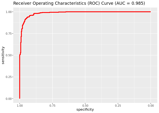
Plotting the ROC curve

``` r
roc_churn <- roc(churn_predictions_ep$churn, churn_predictions_ep$predicted_churn)
```

    ## Setting levels: control = 0, case = 1

    ## Setting direction: controls < cases

``` r
auc_churn <- roc_churn$auc

# Creating ROC plot
ggroc(roc_churn, colour = 'red', size = 1.3) + ggtitle(paste0('Receiver Operating Characteristics (ROC) Curve ', '(AUC = ', round(auc_churn, digits = 3), ')'))
```

![](00_SageMakerAlgo_files/figure-gfm/unnamed-chunk-18-1.png)<!-- -->

Delete the endpoint when done

``` r
model_endpoint$delete_endpoint(delete_endpoint_config=TRUE)
```